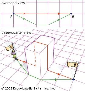
Most people learn geometry in school and assume it’s just about flat surfaces. Triangles add up to 180 degrees. Parallel lines never meet. That is Euclidean geometry. It works fine for your homework. It works okay for building a house. But it fails when you look at the stars or plan a flight path across the Pacific.
Non-Euclidean geometry is simply any system that breaks those flat-surface rules. While the term often gets used as shorthand for hyperbolic geometry, it actually covers any shape where Euclid’s old rules don’t apply. The two big players here are spherical geometry and hyperbolic geometry.
How the Parallel Postulate Changes Everything
The real trouble started with Euclid’s fifth postulate, the one about parallel lines. It says that if you have a line and a point not on that line, there is exactly one line through the point that runs parallel to the first.
For centuries, mathematicians hated this rule. It felt clunky. It didn’t seem as “self-evident” as the others. They spent 2,000 years trying to prove it using the other four postulates. They failed.
Eventually, two men stopped trying to prove it and started playing with what happens if you remove it. Nikolay Lobachevsky in Russia and János Bolyai in Hungary independently published their findings around 1829 and 1831. They discovered a geometry that worked perfectly without the parallel postulate. It was hyperbolic geometry.
Here is how the three systems compare when you change the rules:
- Euclidean: There is exactly one parallel line through the point. The postulate is true. Triangle angles sum to exactly 180 degrees.
- Spherical: There are no parallel lines. Any two “lines” (great circles) will eventually cross. The postulate is false. Triangle angles sum to more than 180 degrees.
- Hyperbolic: There are infinitely many parallel lines through the point. The postulate is false. Triangle angles sum to less than 180 degrees.
The Sky and the Sea: Birth of Spherical Geometry
One branch of non-Euclidean geometry came from looking up. Ancient astronomers needed to track stars and planets against a hemispherical sky. Euclid himself wrote about spherical geometry in his work Phaenomena around 300 BCE.
The other branch came from looking down—or rather, across the ocean. Navigators needed to understand the Earth’s shape to find their way. If the Earth is round, straight lines on a map lie to you. This practical need drove the study of spherical geometry. It wasn’t just theory. It was about not getting lost.
Great Circles Are the New Straight Lines
In spherical geometry, the concept of a “straight line” gets weird. On a globe, the shortest distance between two points is a great circle route. Imagine a string stretched tight between New York and London. That string doesn’t fly in a straight line through the air. It curves along the surface.
Ptolemy noted this in Geography around 150 CE. He wrote that the surface of the land and water is a sphere. Any plane passing through the center of the Earth cuts the surface in a great circle.
These great circles are the “straight lines” of this geometry. They are intrinsically straight. If you walk along one, you aren’t turning. You are moving as straight as possible on a curved surface.
When three of these arcs intersect, they form a spherical triangle. It looks distorted on a flat map. But on the sphere, it’s just a triangle. The difference between triangles on a small sphere and a large one is just scale. In differential geometry terms, spherical geometry is the study of surfaces with constant positive curvature.
Why Maps Lie to You
If spherical geometry is so useful, why don’t we see it everywhere? Because we love flat maps.
Cartographers have to project portions of a sphere onto a flat plane. This is impossible to do without distortion. You can preserve distance. You can preserve area. You can preserve angles. You cannot do all three at once.
The need to balance these trade-offs in mapmaking gave the study of spherical geometry an early, practical boost. It wasn’t just abstract math. It was about representing the world without lying too badly.
The Hidden Geometry of Hyperbolic Space
Then there is hyperbolic geometry. It’s the other half of the non-Euclidean family. It doesn’t match our physical globe. It doesn’t match the flat floor of our classrooms. It describes a space that curves inward, like a saddle or a Pringles chip.
In this space, the rules bend the other way. Lines diverge. Triangles get skinny. Angles shrink. It feels counterintuitive because we don’t experience this shape in daily life. But it exists in mathematics. And later, in physics.
The shift from Euclidean to non-Euclidean wasn’t a sudden revelation. It was a slow unraveling of certainty. Mathematicians had to admit that their “truths” were just assumptions. Assumptions about flatness. Assumptions about parallel lines.
When you drop the parallel postulate, the whole structure shifts. Which path you take—spherical or hyperbolic—depends on whether the space you’re mapping curves back on itself or opens up forever.
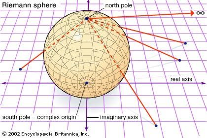
Elliptic geometry is basically spherical geometry with a specific rule tweak. Imagine a globe where the North Pole and the South Pole are treated as the exact same location. That’s the core idea behind the axiomatic formalization of elliptic geometry. It’s not just a theoretical exercise. Bernhard Riemann, a German mathematician, developed an intrinsic analytic view of this in the 1800s. He called it the Riemann sphere. You’ll likely encounter it in university complex analysis courses.
Some textbooks confuse the issue. They label this specific model as Riemannian geometry. That’s misleading. The term Riemannian geometry actually refers to a broader branch of differential geometry. It provides the tools to describe any surface intrinsically, not just the sphere. Stick to the distinction. Elliptic geometry is the formalization of the sphere with antipodal points merged. Riemannian geometry is the framework for studying curved spaces in general.
The Puzzle of Hyperbolic Geometry
If elliptic geometry bends space inward, hyperbolic geometry bends it outward. The first descriptions of hyperbolic geometry emerged from the friction of trying to prove Euclid’s fifth postulate. Mathematicians assumed that if you took away the parallel postulate, you’d get nonsense. Instead, they got a consistent alternative.
It took time to sort out the details. Researchers proved that all hyperbolic geometries differ only in scale. Think of it like spheres. A basketball and a beach ball have the same geometry. They only differ in size. Scale doesn’t change the rules of the space.
By the mid-19th century, the math solidified. It became clear that hyperbolic surfaces must have constant negative curvature. Positive curvature defines elliptic/spherical spaces. Flat, zero curvature defines Euclidean space. Negative curvature is the signature of the hyperbolic type.
But here’s the catch. The equations worked. The logic held up. Yet, mathematicians still couldn’t say for sure if such a surface actually existed in reality. The models were abstract. The question remained: did nature, or even pure mathematics, provide a concrete surface that satisfied these conditions? The existence of the object was still an open question, waiting for a physical or rigorous mathematical construction to prove it wasn’t just a clever fiction.
The Impossible Shape Finally Found
For decades, mathematicians thought they had hit a wall. The problem? Finding a physical representation of hyperbolic geometry that didn’t break the rules of the universe.
It started with Eugenio Beltrami in 1868. He described a surface called the pseudosphere. It had constant negative curvature—the defining trait of hyperbolic space. But it was flawed. Intrinsically straight lines on the pseudosphere intersect themselves. They also hit a bounding circle and stop dead. That’s not how hyperbolic geometry works. Lines there go on forever without looping back or hitting a hard edge.
Then came David Hilbert in 1901. He proved something that effectively killed the project. Hilbert showed you cannot define a complete hyperbolic surface using real analytic functions. Those are the standard, smooth formulas we use to describe shapes. Back then, a surface was an analytic function. Since Hilbert proved it impossible, researchers abandoned the search. The mathematical world accepted the limit.
But the limit was wrong.
In 1955, Dutch mathematician Nicolaas Kuiper proved Hilbert’s limitation didn’t apply to all possible surfaces. He proved a complete hyperbolic surface does exist. It just can’t be drawn with simple, smooth formulas.
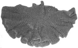
Decades later, in the 1970s, American mathematician William Thurston detailed how to construct it. He didn’t just theorize. He described the actual geometry. And here is the strange part: you don’t need a supercomputer to build it.
You can crochet it.
Why Crochet Changes the Game
Thurston’s hyperbolic surface isn’t just a theoretical object. It is tangible. If you follow specific crochet patterns, you create a physical model of infinite, negative curvature.
Why does this matter? Because it turns an abstract proof into something you can hold. The hyperbolic crochet technique uses increasing stitches to force the fabric to curve outward. Each row adds more material than the last, creating that flared, wavy look characteristic of hyperbolic geometry.
It’s not just a craft project. It’s a direct application of Kuiper’s existence proof. It’s Thurston’s construction made real.
From Pseudosphere to Practical Model
The journey from Beltrami’s incomplete pseudosphere to the crocheted hyperbolic surface shows how mathematical definitions evolve. We moved from:
- 1868: The pseudosphere (incomplete, self-intersecting)
- 1901: Hilbert’s impossibility proof (based on smooth functions only)
- 1955: Kuiper’s existence proof (broadening the definition of surface)
- 1970s: Thurston’s construction (practical, visualizable models)
Today, students and artists use crochet to visualize these complex concepts. It’s a concrete way to grasp negative curvature. No advanced calculus required. Just yarn and a hook.
The shape exists. It’s complete. And it’s in your hands.
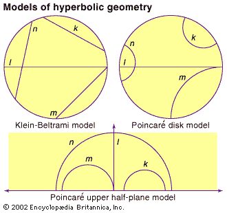
Flat maps of the Earth are always a lie. They stretch, shrink, and tear to fit a sphere onto paper. Hyperbolic geometry faces the same problem. You cannot flatten a saddle-shaped surface without breaking something. Yet, in the 19th century, mathematicians didn’t give up. They built three distinct models to map this curved reality. These aren’t just abstract puzzles. They are tools. Use them together, and the invisible shape of hyperbolic space starts to make sense.
The story really kicks off between 1869 and 1871. Eugenio Beltrami and Felix Klein, a German mathematician, cracked the code. They created the first complete framework for what they literally named “hyperbolic” geometry. Before this, the concept was shaky. Now, it had a house.
The Straight Line Paradox in the Klein-Beltrami Model
Look at the top left of the reference figure. That’s the Klein-Beltrami model. It squeezes the entire hyperbolic plane into the inside of a circle. Simple, right?
Here is the catch. In this model, straight lines—called geodesics in the hyperbolic world—become straight chords in the circle. If you want to go from point A to point B, you draw a straight line. It looks Euclidean. It feels familiar.
But there is a tax for this comfort. The model preserves “straightness” but ruins angles. Things that should be ninety degrees look skewed. It’s a map that tells you exactly which way is north, even if the landscape looks warped.
Curved Paths and Preserved Angles
Fast forward to about 1880. Henri Poincaré, a French mathematician, enters the chat and throws two more models into the ring. These are different. Much more different.
First, the Poincaré disk model (top right). Again, we are looking at a circle. But the rules change. Geodesics are no longer straight lines. They are circular arcs. Or diameters. These arcs hit the outer boundary of the circle at perfect right angles.
Why does this matter? Because Poincaré didn’t just want to show the shape. He wanted to preserve angles.
In the Poincaré disk, local geometry looks just like the flat Euclidean plane, even if the global structure is wildly different.
This is called conformality. Distances are stretched. The edges of the disk are infinitely far away. But if you measure an angle with a protractor, it reads correctly. For tasks involving navigation or optical illusions, this is the gold standard.
The Infinite Upper Half-Plane
The third model is the Poincaré upper half-plane model (bottom of the figure). Forget the circle. Here, the hyperbolic surface maps to the entire half-space above the x-axis.
Geodesics here are semicircles or vertical rays. They always meet the x-axis at right angles. It’s a clean, linear layout.
Like the disk model, this setup distorts distance. The closer you get to the x-axis, the more space expands. But again, angles are preserved. If you draw