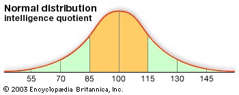
You have probably seen it before. That smooth, symmetrical bell shape that pops up in everything from standardized test scores to quality control reports. It is the normal distribution. Also known as the Gaussian distribution. It is the most common way independent random variables behave.
The curve is defined by two main numbers. The mean sits at the top. It is the average. The graph mirrors itself perfectly around this center point. Then you have the standard deviation. This number decides how wide or narrow the curve gets. A small standard deviation creates a steep, tall graph. A large one makes it flat and wide.
The math behind it relies on an exponential function. The formula uses e, which is roughly 2.718. It also uses your mean (μ ) and the standard deviation (σ ). The total area under this curve always equals one. This is not a coincidence. It is by design. Because the area is normalized to unity, you can read probabilities directly from the space under the line. An area of 0.5 means a 50% chance.
Historically, calculating these areas required heavy calculus. Most people did not have time for that. So, in the 19th century, statisticians made tables. These were for the standard normal distribution. That is where the mean is zero and the standard deviation is one. If your data did not match those numbers, you had to rescale it. You subtract the mean. Then divide by the standard deviation. The formula looks like this: (x – μ ) / σ.
Calculators have mostly killed those paper tables. You punch in your numbers and get the answer instantly. But the concept remains vital for understanding probability theory.
The name “Gaussian” comes from Carl Friedrich Gauss. He was a German mathematician. In 1809, he developed the two-parameter exponential function. He was trying to understand errors in astronomical observations. This work helped him create the law of observational error. It also advanced the method of least squares approximation.
Another early user was James Clerk Maxwell. He was a British physicist. In 1859, he used this distribution to describe molecular velocities. His work later became the Maxwell-Boltmann distribution law.
Long before Gauss, Abraham de Moivre got the ball rolling. In his 1718 book Doctrine of Chances, he noticed something interesting. Probabilities for discrete events—like flipping coins or rolling dice—could be approximated by an exponential curve. Pierre-Simon Laplace took this further. In his 1812 work Théorie analytique des probabilités, he generalized de Moivre’s idea. He created what we now call the central limit theorem.
This theorem is powerful. It proved that almost all independent random variables converge to a normal distribution as your sample size grows. The convergence happens rapidly. This discovery allowed mathematicians to solve problems with calculus that were previously impossible. It turned discrete problems into continuous ones. It made intractable issues manageable.
So why does this matter to you? If you are taking a stats class, you will use this every day. If you are a researcher, your data likely follows this pattern unless it does not. It is everywhere. It is the default assumption for many statistical tests.
The beauty of the normal distribution is its universality. It does not care what you are measuring. It only cares that you are measuring independent variables. The central limit theorem ensures that even if your raw data is messy, the averages will smooth out into a bell curve. This is why we can make predictions about large groups based on smaller samples.
There is a reason this curve is so familiar. It is not just a mathematical curiosity. It is a fundamental property of randomness. When enough independent factors come together, the result tends toward this shape. It is a bit like entropy. Disorder leads to a predictable pattern.
Does your data fit the curve? That is the first question you should ask. If it does, you have tools to analyze it with ease. If it does not, you need different methods. The normal distribution is not a law of nature. It is a model. A very useful one. But sometimes reality refuses to fit the bell.
We rely on these models to make sense of chaos. The central limit theorem gave us that power. It turned uncertainty into something calculable. Gauss and Maxwell did not set out to create a universal statistical tool. They just wanted to understand stars and gas molecules. But their work revealed a deeper truth about how the world aggregates random events.
Next time you see a bell curve, remember the history. Remember de Moivre’s coins and Laplace’s theorems. It is not just a shape. It is the result of centuries of trying to find order in randomness. The curve simplifies the complex. It allows us to predict the unpredictable.
But keep in mind. Real data is rarely perfectly normal. Skewness and kurtosis exist. The tails are often heavier than the model predicts. The normal distribution is an approximation. A powerful one. But an approximation nonetheless. Understanding its limits is just as important as understanding its application. That is where the real insight lies.